Putting way too much thought into choosing a reasonable delay for a suspend-then-hibernate policy
I am an inconsistent laptop user. Sometimes I shut the lid and pick it back up an hour later. Sometimes I don't touch it for a week. The latter behavior is annoying, because I often returned to a completely dead machine, losing both whatever I was in the middle of working on and dealing with the inconvenience of having to plug it in. The culprit (other than me) is that a sleeping laptop still drains the battery -- in my case, somewhere around 1% an hour, or so. Combine multi-day sleeps with a partially full battery and it's easy to end up with a dead machine.
There is solution to this, but to place it in the appropriate context we need to understand what the laptop is actually doing when we put it to sleep. The standard behavior, which I will refer to as suspend is to more or less freeze the system state and place as many components into a low power state as possible.1 We can contrast this with hibernate, where the system state is frozen, saved to disk, and then the system is powered off entirely. Hibernation trades significantly longer wake times - closer to a cold boot - for near-zero power drain.2
Considering these two as totally distinct options, the trade-off is difficult to make. A laptop set to hibernate every time the lid is closed would be inconvenient to use for most people. Not to mention there is a disk wear cost to saving system state to disk every time you want to put the machine to sleep. The solution is to combine the two sleep strategies in a mode provided on Linux by systemd called suspend-then-hibernate.
In the suspend-then-hibernate mode, the system is first suspended and an RTC
alarm is set to wake the system after a delay and place it into hibernation.
This hybrid mode maintains fast wake-ups for short sleeps and the eventual
hibernate prevents long sleeps from fully draining the battery. The main
question to be answered about this mode is how long do you wait before
hibernating the system?.
The default behavior estimates the battery drain while asleep and attempts to set the timer to prevent the system from dropping much below 5% battery. This policy helps avoid the problem of coming back to a completely dead laptop, but does little to actually prevent significant sleep drain. For example, leaving your laptop for a few days under this default policy may prevent you from losing your in-progress work, but you will still need to immediately charge when you go to use the system again.
The alternative that I am going to explore here is setting a delay timer based on my own particular laptop usage patterns and explicitly explore the trade-offs between battery savings and inconvenience due to hibernate wake times.
To choose an appropriate delay timer, I need to evaluate what the effects of setting that timer would have been. To this end, I am going to focus on two quantities.
The first of these I am calling "average awake battery time", which I am defining as the amount of actual usage time I get out of a full charge. If my active battery drain is 10% per hour, but typical usage means that 30% of the battery is lost while sleeping, then my "awake battery time" is 7 hours. This tries to capture how much use I get out of my machine in between charges. We want this number to be high.
The other side of this is the "fraction of wake events that are fast" and by fast I mean waking from a suspend state. We also want this number to be high. You can see that an always-suspend policy is at one extreme -- 100% fast wake-ups but minimum awake battery time -- and an always-hibernate policy is at the other extreme -- 0% fast wake-ups and maximum awake battery time.3
The decision we need to make is selecting , the delay timer for when a sleeping laptop transitions from transitions from suspend to hibernate.
We will perform this evaluation via simulation, assuming that we know a few key parameters about the system. The approach will be to simulate the energy drain across multiple sleep-wake cycles by drawing awake and sleep durations from my historical data. The rough sketch is as follows:
- Assume that the laptop starts awake at 100% battery, let be the chosen hibernate delay timer, and start with .
- Draw a duration of awake usage, , from historical data.
- Assume the battery drains according to awake power usage, , meaning the energy loss from the first wake usage is .
- Draw a sleep duration, , from historical data. Assume battery drains according to average suspend power usage, , for all time when and according to average hibernate power usage, for all time when . This results in a total sleep power draw of , where is 0 when and is the energy cost associated with entering and leaving a hibernate state.
- Increment and repeat from step 2 until the battery is depleted. If the battery is depleted during a wake cycle, be sure to use the drain time and not the full value for that cycle. We can then add up the total amount of time the system was awake across all the sleep wake cycles to get the "awake battery time"
- Repeat simulation many times to get multiple "awake battery time" values and average to get our metric.
The "fast wake fraction" can be computed directly from the historical data as the fraction of historical sleep events that are less than .
The simulation described above depends on having access to some key information about our system. The first is historical data on wake and sleep durations, which I have logged over the last few months. The second are the various energy parameters that I described in the simulation sketch, these we will have estimate statistically.
We are going to build up our modeling of this process bit by bit, but first we need to talk about the data collection process. I rely on a battery monitoring utility that collects the reported battery level (in milliwatt-hours) and the timestamps of transitions between various systems states, e.g. awake -> sleep -> hibernate -> awake. The system state transitions are ultimately sourced from kernel logs and we will consider them accurate.
There are two quirks to keep in mind about the battery readings. First, the battery reports energy levels only to the granularity of 10 mWh. This is quite small and makes little difference for measurements of power draw when awake, but has a real effect on estimating power drain during suspend or hibernation. Second, the battery readings only occur once a minute while the system is awake. There is no guarantee that the state transitions timings will align closely with those energy readings. The drawing below shows what can happen:
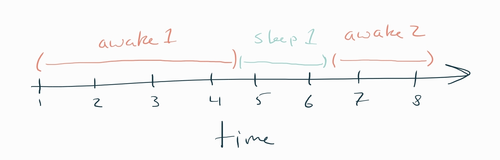
If we assume that energy readings are taken at each time step, we see that the state transitions happen in between energy readings. Since no readings are taken while the system is asleep, we do not get readings at times 5 and 6. We need to handle these quirks in our modeling.
We start by estimating the awake power draw by itself. For this, we will collect a dataset of the first and last energy reading made during an awake period (being careful to exclude any cases when the system is not in a "Discharging" state) and the corresponding timestamps of those measurements.
For a given wake period, let and be measurements of the battery energy levels. Due to the minimum granularity of 10 mWh that these measurements can take, we will assume that there are latent true energy values of and . I will make the assumption that the measurements represent rounded values, so the true value is within mWh. We can represent our uncertainty about the true values as a uniform distribution over that region:
Conditional on knowing the true values, then the average power draw during a given wake period is given by . We can then estimate:
where is expected awake power usage, our target parameter to estimate, and is the standard deviation of awake power draws. The Stan code for this model is:
data {
  int<lower=1> N_readings;

  // energy measurements (mWh)
  vector<lower=0>[N_readings] E_hat;
  // timestamps of readings (hours)
  vector<lower=0>[N_readings] T;

  // Energy measurement granularity
  real<lower=0> G;

  // Number of awake periods
  int<lower=1> N_awake;

  // Indexes of (initial, final) energy readings
  array[N_awake, 2] int<lower=1, upper=N_readings> Awake_Index;
}
transformed data {
  vector<lower=0>[N_awake] DeltaT = T[Awake_Index[ : , 2]]
                                    - T[Awake_Index[ : , 1]];
}
parameters {
  // Latent true energy values
  vector<lower=E_hat - G / 2, upper=E_hat + G / 2>[N_readings] E;

  real<lower=0> delta_a;
  real<lower=0> sigma_a;
}
transformed parameters {
  vector<lower=0>[N_awake] DeltaE_awake = E[Awake_Index[ : , 1]]
                                          - E[Awake_Index[ : , 2]];
}
model {
  delta_a ~ normal(5000, 2000);
  sigma_a ~ normal(2000, 1000);

  DeltaE_awake ~ normal(delta_a * DeltaT, sigma_a * DeltaT);
}
The priors I placed on and represent a guess at average power draw around 5W with quite wide uncertainty ranges -- enough to weakly constrain these values to a plausible range. Sampling from this model with my collected data (, I get the following posterior summary:
| Parameter | Mean | 5% | 50% | 95% |
|---|---|---|---|---|
| 5914 | 5671 | 5914 | 6167 | |
| 911 | 740 | 899 | 1118 |
Based on the data I have collected, my average power draw while the system is awake is somewhere in the ballpark of 5.6 to 6.2 W.
To move this analysis towards estimation of the power draw associated with sleep states, we need to extend this model to account for energy drain as the system transitions from awake to suspend and hibernate. The following diagram shows how the energy measurements we take compare to the system state transitions.
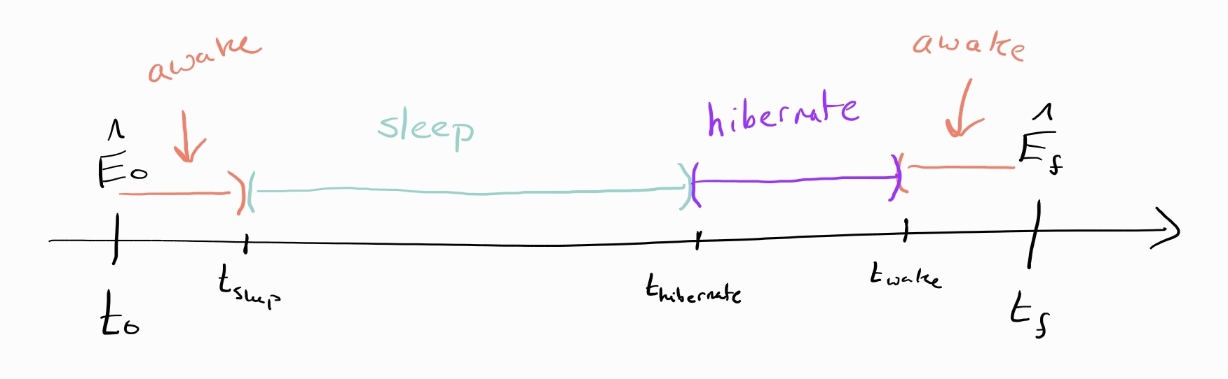
Importantly, we have each labeled point in this diagram as data. We know when each energy measurement is taken as well as when the system initially goes to sleep, when it transitions to hibernate (if it does), and when the system wakes back up. What is needed from here is to relate these known times and energy observations to our parameters of interest.
As before, we will work directly the latent and values. We will assume that when the system is in each of the different states that the power draw is sampled from a normal distribution with mean and standard deviation according to that particular state parameter, e.g. . Since we will treat power draw in each state as independent, we can add up the total energy usage and will end up normally distributed.
Let's first consider the non-hibernation case the system goes from
awake -> suspend -> awake. The system is in an awake state for a
total time equal to
and in a sleep state for . Note, I am
going to assume that the awake drain at the start and end here share the
same average power drain (I can't be bothered to separate them). In
this case, we get:
The awake -> suspend -> hibernate -> awake case follows much a similar form
except we introduce and add a
constant to the mean that represents the additional energy cost of
entering and resuming from the hibernate state, which is more intensive than a
suspend process. The time spent while awake is the same as before, but time
while asleep is and time spent in hibernate is . Then we get:
With these in hand, we can extend the initial model we built for the awake-only case to handle the various sleep cases as well. The Stan code for the full model is:
data {
  int<lower=1> N_readings;

  // energy measurements (mWh)
  vector<lower=0>[N_readings] E_hat;
  // timestamps of readings (hours)
  vector<lower=0>[N_readings] T;

  // Energy measurement granularity
  real<lower=0> G;

  // Number of awake periods
  int<lower=1> N_awake;

  // Indexes of (initial, final) energy readings
  array[N_awake, 2] int<lower=1, upper=N_readings> Awake_Index;

  int<lower=0> N_sleep;
  // Indexes of the last reading before sleep and first reading after wake.
  array[N_sleep, 2] int<lower=1, upper=N_readings> Sleep_Index;

  // Transition times
  vector<lower=0>[N_sleep] T_sleep;
  vector<lower=0>[N_sleep] T_wake;
  vector<lower=0>[N_sleep] T_hibernate;
  array[N_sleep] int<lower=0, upper=1> Hibernated;
}
transformed data {
  vector<lower=0>[N_awake] DeltaT = T[Awake_Index[ : , 2]]
                                    - T[Awake_Index[ : , 1]];
  vector[N_sleep] DeltaT_sleep_awake = rep_vector(0, N_sleep);
  vector[N_sleep] DeltaT_suspend = rep_vector(0, N_sleep);
  vector[N_sleep] DeltaT_hibernate = rep_vector(0, N_sleep);

  if (N_sleep > 0) {
    for (n in 1 : N_sleep) {
      real t0 = T[Sleep_Index[n, 1]];
      real tf = T[Sleep_Index[n, 2]];
      real sleep_duration = T_wake[n] - T_sleep[n];
      DeltaT_sleep_awake[n] = (T_sleep[n] - t0) + (tf - T_wake[n]);
      if (Hibernated[n] == 1) {
        DeltaT_suspend[n] = T_hibernate[n] - T_sleep[n];
        DeltaT_hibernate[n] = T_wake[n] - T_hibernate[n];
      } else {
        DeltaT_suspend[n] = sleep_duration;
      }
    }
  }
}
parameters {
  // Latent true energy values
  vector<lower=E_hat - G / 2, upper=E_hat + G / 2>[N_readings] E;

  real<lower=0> delta_a;
  real<lower=0> sigma_a;
  real<lower=0> delta_s;
  real<lower=0> sigma_s;
  real<lower=0> delta_h;
  real<lower=0> sigma_h;
  real<lower=0> Delta; // fixed hibernate entry/resume cost (mWh)
}
transformed parameters {
  vector<lower=0>[N_awake] DeltaE_awake = E[Awake_Index[ : , 1]]
                                          - E[Awake_Index[ : , 2]];
  vector<lower=0>[N_sleep] DeltaE_sleep = E[Sleep_Index[ : , 1]]
                                          - E[Sleep_Index[ : , 2]];
  vector[N_sleep] mu_sleep = rep_vector(0, N_sleep);
  vector<lower=0>[N_sleep] sd_sleep = rep_vector(0, N_sleep);
  if (N_sleep > 0) {
    for (n in 1 : N_sleep) {
      // Note in the below DeltaT_hibernate is 0 in sleep-only
      mu_sleep[n] = delta_a * DeltaT_sleep_awake[n]
                    + delta_s * DeltaT_suspend[n]
                    + delta_h * DeltaT_hibernate[n] + Hibernated[n] * Delta;
      sd_sleep[n] = sqrt(
                         square(sigma_a * DeltaT_sleep_awake[n])
                         + square(sigma_s * DeltaT_suspend[n])
                         + square(sigma_h * DeltaT_hibernate[n]));
    }
  }
}
model {
  // Power means and SDs are in mW, energies in mWh, durations in hours.
  delta_a ~ normal(5000, 2000);
  sigma_a ~ normal(2000, 1000);
  delta_s ~ normal(500, 400);
  sigma_s ~ normal(200, 100);
  delta_h ~ normal(50, 50);
  sigma_h ~ normal(20, 20);
  Delta ~ normal(100, 100);

  DeltaE_awake ~ normal(delta_a * DeltaT, sigma_a * DeltaT);
  DeltaE_sleep ~ normal(mu_sleep, sd_sleep);
}
Fitting this model with our additional sleep data, comprised of 23 suspend-then-hibernate events and 10 suspend-only events, plus the original 35 awake events, we get the following posterior summaries:
| Parameter | Mean | 5% | 50% | 95% |
|---|---|---|---|---|
| 6015 | 5749 | 6016 | 6283 | |
| 1019 | 832 | 1009 | 1236 | |
| 284 | 262 | 283 | 307 | |
| 32 | 22 | 32 | 44 | |
| 9.3 | 4.0 | 9.2 | 14.8 | |
| 4.8 | 0.5 | 4.3 | 11.1 | |
| 168 | 83 | 169 | 246 |
Our awake parameters shifted up a bit from our initial model since each sleep event includes some awake time, but ends up in more or less the same spot.4 Suspend power draw at a mean of 284 mW and hibernate power draw trickles at around 9 mW. The mean value lands at 168 mWh, which with my battery reporting at 41900 mWh capacity hits around 0.4%, which isn't nothing.
This model output gives us all the information that we need to run our full simulation at different values and compute the quantities of interest.
With historical data on my sleep and awake usage patterns, we can proceed with the simulation as described above. To handle uncertainty in the power drain parameters, we draw their values for each simulated full battery drain from the joint posterior defined by the Stan model above.5
The simulation results are presented in the graph below, where we plot the empirical fast wakeup fraction and simulation average awake time at different values of .
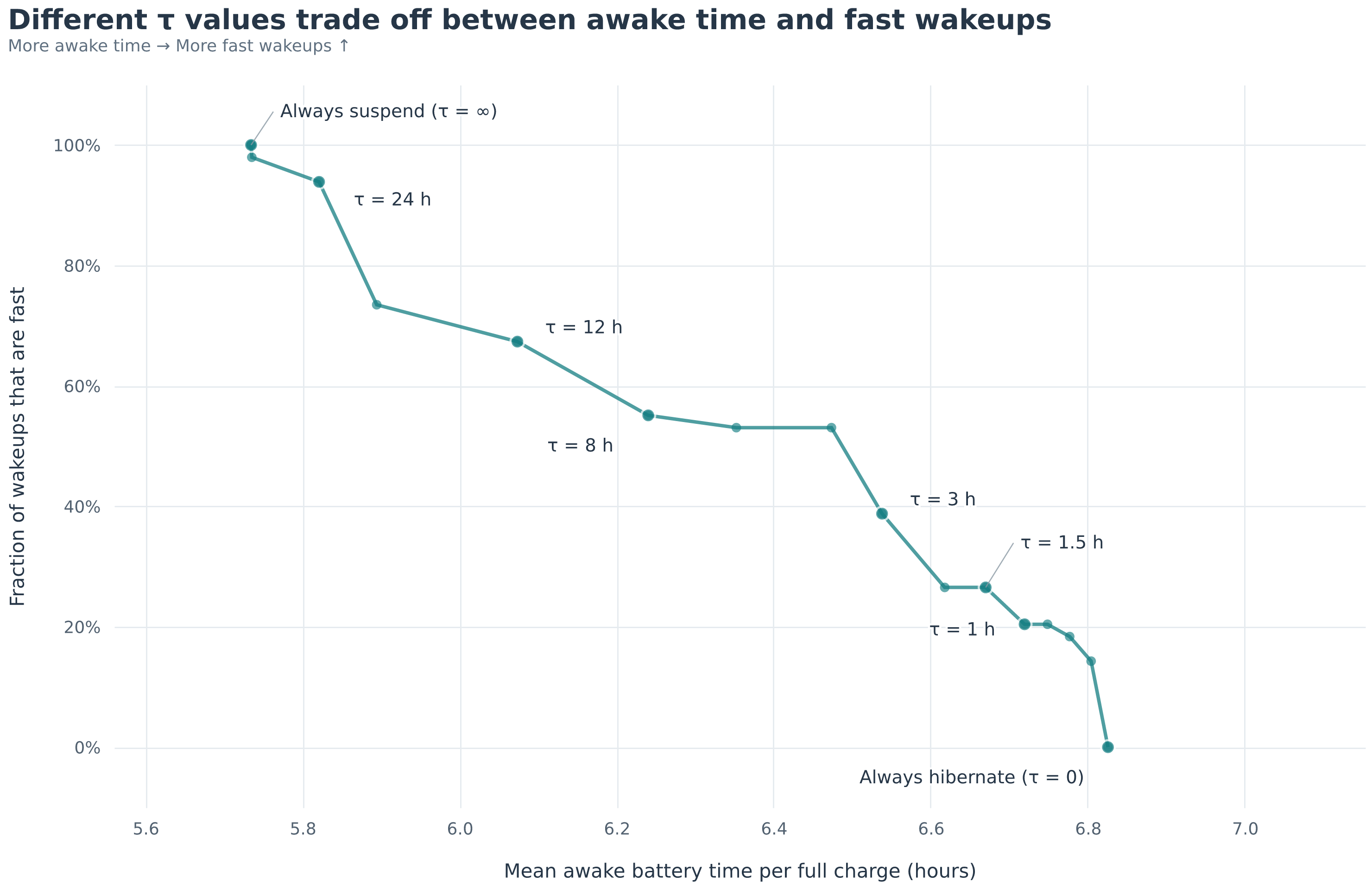
The general trends we see are as expected: more aggressively hibernating by decreasing increases the awake battery time at the cost of fewer fast wake-ups. The awake battery time ranges from about 5.7 hours in the always-suspend case to 6.8 hours in the always-hibernate case, suggesting that there is up to a 20% increase in practical battery life that we could get by choosing different values. Interestingly, the landscape is not smooth. We see a few regions where the curve plateaus and additional awake battery life can be gained without sacrificing fast wake-ups.
As with many multi-objective optimization problems, the trade-offs between the two quantities here are not obvious. How much one wants to tolerate a slow hibernate wake versus potential loss in average awake battery time is a personal decision. However, what is definitely useful for me is to see those trade-offs explicitly laid out.
Personally, I don't mind a hibernate wake that much, especially if it comes after a long sleep period, like overnight. The histogram below shows the distribution of sleep durations that I have logged as part of this effort.
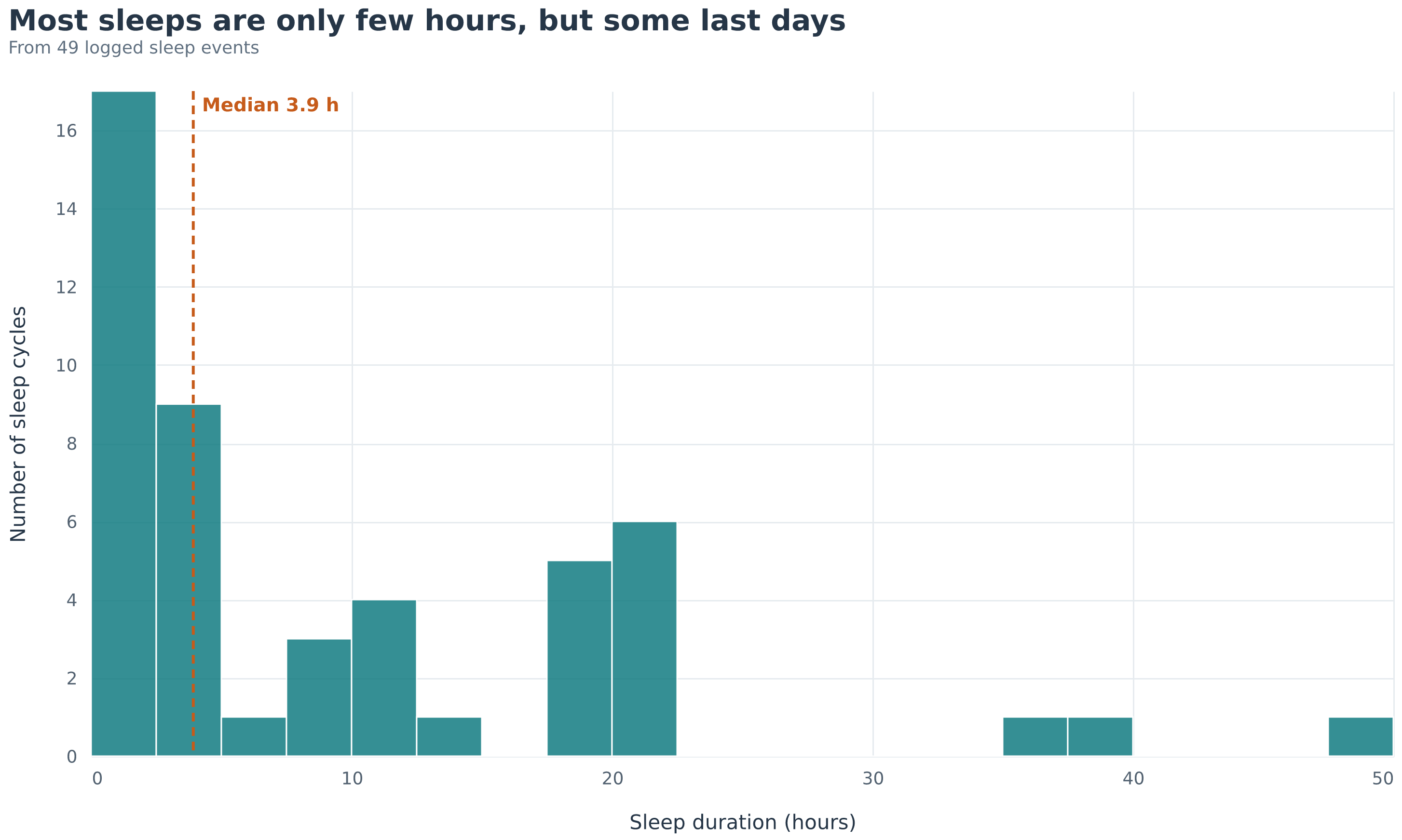
From 49 logged events, we see the biggest spike of events in the 0-5 hour range with other notable bumps around 8-12 and 18-22 hours. I know that when I use my laptop, short breaks of an hour or so are common but when I put it down for the evening, I'm not going to pick it back up until the next morning or later that day (or longer).
The dip between the modes below 5 and around 10 corresponds to the long plateau we see in the simulation results where decreasing gets us awake battery life more or less for free. From these results, the setting seems to be an excellent middle-ground where we retain fast wakes for common short sleep events, but raises the awake battery life to nearly 6.5 hours, which is about 70% of the way to the always-hibernate maximum.
I found this exploration interesting for a few reasons. For one, it was a very practical investigation into what kind of actual battery life I get as represented by awake time between charges. My 2019-era Thinkpad is hardly a top-of-the-line machine in 2026, but around 6 hours of usage time between charges is enough to get me through most things. However, stretching that time a little bit can go a long way towards improving my actual experience using the machine.
I enabled the 4 hour suspend-then-hibernate timer over the few days that I have been chipping away at writing this post, and I feel like I already notice a difference. In particular, it seems less common that I wake up my laptop and the first thing I need to do is charge (which was very annoying).
The second thing is that in my typical usage patterns, a solid hour of possible awake time was being lost to power drain while sleeping. With my chosen setting, I get somewhere around an addition 45 minutes of usage while retaining over half of my fast wakes, a pretty significant difference!
As to how this analysis and these results would translate to other cases, I cannot say. The outcomes were based on my particular sleep-wake patterns and my particular hardware's power profile. My tendency to have shorter sessions spread across multiple days made sleep drain a relatively large fraction of overall battery drain, and as a result, dropping into hibernate after a few hours usefully extends usage time. Someone who uses their machine for longer sessions or has a laptop with significantly lower sleep drain wouldn't get as much benefit.6
-
There are finer distinctions to be made. On Linux, the S3 or Suspend-to-RAM sleep state saves the system state in RAM, keeping it powered, and attempts to switch the rest of the machine to low power states. A similar, more modern approach is called s2idle or Suspend-to-Idle, which keeps the system in a partially awake low-power state. Both states tend to have significantly lower power draw than an active system, but s2idle has near-instant wakes whereas S3 can take a few seconds. Whether a particular machine supports one or both of these states is hardware dependent and varying quality of implementations can result in one or the other being better in terms of sleep power draw. For our purposes, we will treat them as equivalent and just refer to them as "suspend". ↩
-
Hibernation, as I have learned, is somewhat controversial in some Linux communities. It can be very finicky to get working depending on your particular hardware, there are security concerns with serializing memory to disk, and it often requires manual setup that can be obscure for less savvy users. For my purposes, I have had a good experience with it and won't wade into any of those larger conversations. ↩
-
Technically, there are usage patterns where always hibernating is worse than suspending. Since the process of entering and waking from hibernate is more expensive than just suspending, a pattern of many short 15 minute sleeps would probably lose more battery than just suspending. In practice, it serves as something like an upper bound. ↩
-
There's a reasonable argument to be made that the power draw during the "awake" segments is materially different than the power draw in the time just before and just after a sleep segment. Since the parameter summaries don't shift that much and it would be a good deal of work to dig into that fine distinction, I'm not going to concern myself too much with it. ↩
-
The way I handle this in the simulation is mostly for convenience. It's slightly different than how we actually modeled it, but at the end of the day I am really only going to look at the mean outcomes. Also, this is a blog post, the standards aren't that high. ↩
-
I think it would be possible to build an adaptive version of this analysis, where usage and battery data is collected to automatically tune a suspend-then-hibernate delay timer. I started looking into this, because it is feasible to make this timer dynamic, e.g. a system that knows that putting my laptop to sleep at midnight should demand a more aggressive hibernate timer than doing so at 4 PM. The reality is that the always-hibernate battery life is a practical upper bound on what such a system could save. I didn't want to go through all the effort to save maybe another 10-15 minutes on average. ↩